This article will review statistical hypothesis testing in general and then introduce equivalence testing and its application.
What is equivalence testing and when should we use it?
Most quality professionals are familiar with basic hypothesis tests such as the 2-sample t test. However, depending on the goals of the study, another type of test, called an equivalence test, may be utilized instead of traditional hypothesis tests. This article will review statistical hypothesis testing in general and then introduce equivalence testing and its application. To illustrate the differences between traditional hypothesis tests and equivalence tests, we will focus on the case of comparing 2 independent samples. The concepts may be easily extended to other situations (such as comparing a sample to a target or paired comparisons).
Standard Hypothesis Testing
WinSPC Means Lower Costs and Higher Quality
WinSPC is software to help manufacturers create the highest quality product for the lowest possible cost. You can learn more here.
Every day we are faced with uncertainties when making decisions. For example:
- Which route should I drive to work today?
- Which entrée should I pick from a restaurant menu?
- Should I purchase a specific stock for my portfolio?
Because we ordinarily cannot know future outcomes in advance, we typically weigh the probabilities and benefits of making a correct decision and the potential adverse outcomes if we are wrong. When data is available, it becomes easier to make good, objective decisions while minimizing the risks of making an incorrect decision.
Formal statistical hypothesis testing involves the establishment of a statement called the null hypothesis. The null hypothesis represents the status quo and is assumed to be true unless countered by the data. The alternate hypothesis is typically the opposite conclusion and is usually what the experimenter is trying to claim (if the data supports it). So the result of a hypothesis test is either:
- A rejection of the null hypothesis (in which case we believe the alternate hypothesis is true at the specified confidence level)
- A failure to reject the null hypothesis (in which case we conclude that there is insufficient evidence to claim that the alternate hypothesis is true at the specified confidence level)
Note that in the second potential outcome, we do not conclude that the null hypothesis is true just because we fail to reject it.
An Analogy
In the classic analogy of the criminal justice system in the United States, the null hypothesis is that the accused is “innocent” and the alternate hypothesis is that the accused is “guilty”. In other words, the accused is presumed to be innocent unless enough convincing evidence is presented to result in a conviction. A “not guilty” verdict (e.g. failure to reject the null hypothesis) does not necessarily imply that the jury believes the accused is innocent. Rather, it means that the evidence presented was insufficient to conclude the accused is guilty beyond a reasonable doubt. Some or all of the jury may believe that the accused is probably guilty, but some reasonable doubt exists so they do not convict per the decision criteria explained to them.
What about Mistakes?
Of course errors are possible in any decision and properly designed hypothesis tests will minimize both types of errors that may occur. The potential errors are classified as follows:
- Type I error – The null hypothesis is rejected when it shouldn’t be (probability is α)
- Type II error – The null hypothesis is not rejected but it should be (probability is β)
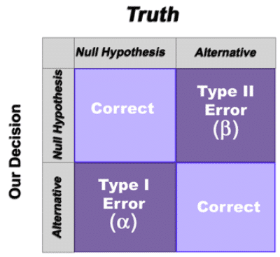
In our analogy, a Type I error occurs when an innocent person is found guilty and a Type II error occurs when a guilty person is not convicted. Naturally, attempts to minimize one type of error will lead to more errors of the other type (all other things being held equal). So attempts are made to judge the severity of each error in a given situation to appropriately balance the risks.
In the practice of standard hypothesis testing, the Type I error is explicitly specified and determines the confidence level if the null hypothesis is rejected. Often, this is set around 0.05 (or 5%), but it can be any probability. The Type II error depends on several other factors: sample size, the actual difference in what we are testing, the confidence level, and the Type I error. In the practice of standard hypothesis testing, the Type II error should be understood and managed by the selection of an appropriate sample size. This is often not well understood or is overlooked. This is the key reason why equivalence tests may be more appropriate than standard hypothesis tests.
Comparing 2 Independent Samples
It is often necessary to compare 2 or more groups of data to determine whether they are statistically and practically the same or different. Some examples include:
- Compare measurement data from two different measurement devices to assess whether they are the “same” or not
- Compare average weights of food products being filled at different filling stations
- Compare means or standard deviations of a key characteristic from two different suppliers
- Compare parts coming from multiple cavities or filling heads
When comparing the averages of two independent groups of data, most quality professionals or six sigma personnel will utilize a 2-sample t test. The hypotheses for the 2-sample t test are as follows:
The mathematical details of the 2-sample t test are not covered here. However a key point is that the ability to detect differences in averages depends on both the difference between the sample averages and the variation within each group. Statistical software will provide a p-value which allows us to determine whether or not we have sufficient evidence to reject the null hypothesis. In short, if the p-value is less than the significance level (α), then we reject the null hypothesis with (1-α)% confidence. For example if α is 0.05, then we reject the null hypothesis if the p-values is less than 0.05 (at a confidence level of at least 95%). As we saw earlier, α is also the probability that a Type I error is made.
Suppose we obtain a p-value of 0.23? Should we conclude that the two means are equal? While it may be tempting to do so, this conclusion is not valid. Remember, we can only conclude whether there is enough evidence to reject the null hypothesis or not. Failure to reject it does not imply that it is true. It’s very possible that the test had insufficient power to result in a rejection of the null hypothesis (e.g. due to limited sample size or large variability in the data). So the failure to reject the null hypothesis does not lead to a conclusion that the process means do equal each other.
We can only state that there is insufficient evidence to conclude that a difference exists. Hopefully at this point, it is clear why a 2-sample t test is not the best choice if we are actually trying to demonstrate equivalence between two groups. Only if we are trying to demonstrate a difference between the two groups (e.g. one drug produces a superior response to another), does the 2-sample t test foot the bill.
Finally…..Equivalence Tests
Tests that allow us to conclude equivalence (e.g. two process averages are equal) with a specified confidence level are called
equivalence tests.
When using equivalence tests, we must specify how large of a difference between the group averages would represent a practically important difference. Then, smaller differences than that are considered insignificant when comparing the group averages and equivalence may be concluded. The interval around 0 that represents the biggest true difference between the group means that we will accept while still calling the group averages equivalent is called the equivalence interval . For example, a manufacturer of surgical needles measures the penetration force to cut through tissue. Perhaps a difference between lot averages that falls between -5 and +5 grams may be considered insignificant. Thus, the equivalence interval is (-5,+5).
The hypothesis test for equivalence can be written as follows:
H0: The difference between the two group means is outside the equivalence interval
H1: The difference between the two group means is inside the equivalence interval |
To test for equivalence, two separate hypothesis tests are actually conducted (where the difference refers to the difference between the two group means).
Hypothesis Test 1
H0: The difference is less than or equal to the lower limit for equivalence
H1: The difference is greater than the lower limit for equivalence
Hypothesis Test 2
H0: The difference is greater than or equal to the upper limit for equivalence
H1: The difference is less than the upper limit for equivalence |
In order to conclude equivalence, the null hypothesis for both hypothesis tests must be rejected. If either hypothesis test fails to be rejected, then equivalence cannot be concluded. If both null hypotheses are rejected, then the difference between the group means falls within the equivalence interval and we can claim that the means are equivalent (at the specified confidence level).
Equivalence Test…An Example
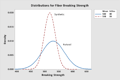
A company is investigating the use of synthetic fibers as a substitute for natural fibers and wants to ensure that the breaking strengths are equivalent. A random sample of 15 natural fibers resulted in an average breaking strength of 530 kg with a standard deviation of 40 kg. A random sample of 12 synthetic fibers provided an average breaking strength of 513 kg with a standard deviation of 20 kg. If the mean breaking strengths are within 20 kg of each other, then the differences in strength are assumed to be negligible.
So the hypothesis test for equivalence is:
H0: The difference between the means is outside the equivalence interval
H1: The difference between the means is inside the equivalence interval |
As indicated earlier, two separate hypothesis tests are performed and these will be illustrated in the software output that follows. The following two curves illustrate the two processes.
Two-Sample Equivalence Test
Equal variances were not assumed for the analysis.
Descriptive Statistics
| Variable | N | Mean | StDev | SE Mean |
| Test | 15 | 530 | 40 | 10.328 |
| Reference | 12 | 518 | 20 | 5.7735 |
Difference: Mean(Test) – Mean(Reference)
| Difference | SE | 95% CI | Equivalence Interval |
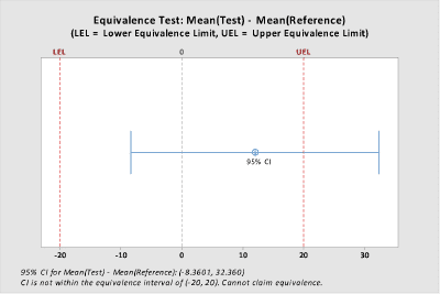
| 12.000 | 11.832 | (-8.3601, 32.360) | (-20, 20) |
CI is not within the equivalence interval. Cannot claim equivalence.
Test
| Null hypothesis: | Difference <= -20 or Difference >= 20 |
| Alternative hypothesis: | -20 < Difference < 20 |
| α level: | 0.05 |
| Null Hypothesis | DF | T-Value | P-Value |
| Difference <= -20 | 21 | 2.7045 | 0.007 |
| Difference >= 20 | 21 | -0.67612 | 0.253 |
Since only one of the hypothesis tests is rejected (p < 0.05), we cannot conclude that the groups are equivalent. The result is also illustrated graphically below. Because the 95% confidence interval around the estimated difference in the group means extends beyond the upper equivalence limit, equivalence is not demonstrated.
Keep in mind that variability is an extremely important consideration in how products perform, so simply comparing means to determine equivalence is only part of the picture.
Power & Sample Sizes for Equivalence Testing
Just as with standard hypothesis testing, we should ensure that the power for the equivalence test is sufficient to reject the null hypothesis and conclude equivalence, if it is in fact true. The power for an equivalence test is the probability that we will correctly conclude that the means are equivalent, when in fact they actually
are
equivalent.
If the equivalence test has insufficient power, we may mistakenly conclude that the means are not equivalent when they actually are. Choosing a sample size to ensure adequate power will be addressed in a future article.
Summary
When the objective of a statistical hypothesis test is to conclude that groups are equivalent, an equivalence test should be utilized. An equivalence test forces us to identify from a practical perspective how big of a difference is important and puts the burden on the data to reach a conclusion of equivalence.
Steven Wachs, Principal Statistician
Integral Concepts, Inc.
Integral Concepts provides consulting services and training in the application of quantitative methods to understand, predict, and optimize product designs, manufacturing operations, and product reliability. www.integral-concepts.com
Download the white paper on how to jump-start a “mini” Six Sigma Quality program on a budget